In this article, I plan to give a high-level explanation of Bi-Directional Path-Tracing and Multiple-Importance Sampling. I also will describe some methods for applying these algorithms into code, and additionally how you might go about writing a path-tracer on the GPU.

This is in no way to be taken as an "be-all end-all" tutorial, nor is it guaranteed to even be mathematically-correct. However, I will add some of my pitfalls in writing a GPU path-tracer.

It's also not designed to be a "line-for-line" programming tutorial. Instead, it's going to loosely describe how you might adapt a renderer to support additional functionality.

In Computer-Science, there are certain problems that don't always adapt to code easily. The classic Uni-Directional Path-Tracing (UDPT) is fairly simple to solve. However, we'll see later that Bi-Directional Path-Tracing (BDPT) is quite a bit more involved.

As long as you trace from the sensor towards the light-source, you're talking about an algorithm that could take less than 30 lines of code to implement.
I'm simplifying a lot here, since in reality there would need to be a framework for casting rays and for defining the scene that those rays intersect.
But still, it's a fairly straight-forward solution.

What I described above is normally referred to as "Eye-Tracing", which is the exact opposite of how light rays propagate in reality.
We refer to its counterpart as "Light-Tracing" which as the name suggests, starts at the light-source and traces towards the sensor.
Light-Tracing requires a bit more planning of how you model your camera (ie: lens, aperture type, and viewing film), but is still relatively simple to implement.

Eye-Tracing is mostly efficient at sampling wide-area lights and open scenes, whereas Light-Tracing is more efficient at sampling tiny lights and also heavily confined/convoluted scenes.
Additionally, Eye-Tracing is nearly incapable of sampling caustics like from glass or mirrors. For that reason, we may prefer to use Light-Tracing for those cases.

The problems start when you try combining these two algorithms together with Bi-Directional Path-Tracing; and then, if you use the more efficient variant, it's called:
Bi-Directional Path-Tracing with Multiple-Importance Sampling (BDPT with MIS).
Whew! That's quite the title for such an important computer-graphics algorithm.
Luckily for us, most people refer to BDPT with MIS as just BDPT since it's hardly used without MIS.
The first term "Bi-Directional" basically means we're tracing rays from both the sensor and the light-source to produce a path.
The second term "Multiple-Importance Sampling" is a method that chooses the best algorithm from many possible candidates.

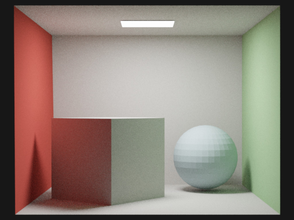
If we consider a single sample in a naive BDPT, we would shoot an eye-ray into the scene, bounce around until a condition is met, and then repeat those steps but from a light-source instead.
After both eye- and light-paths are created, we complete the sample by merging them. This is done by shooting "connection" or "shadow" rays between each vertex in the eye- and light- paths. Once all eye-vertices have been connected to every light-vertex, then the sample is complete. We repeat these steps for the rest of the image.

At this point, BDPT may sound quite complicated, but it can be further broken down into smaller problems. We can treat each of the eye-to-light path connections as if an eye-path was sampling a light-source.
In this case, however, the lights are substituted with light-vertices instead, which contain the required information of their contribution to the sample.

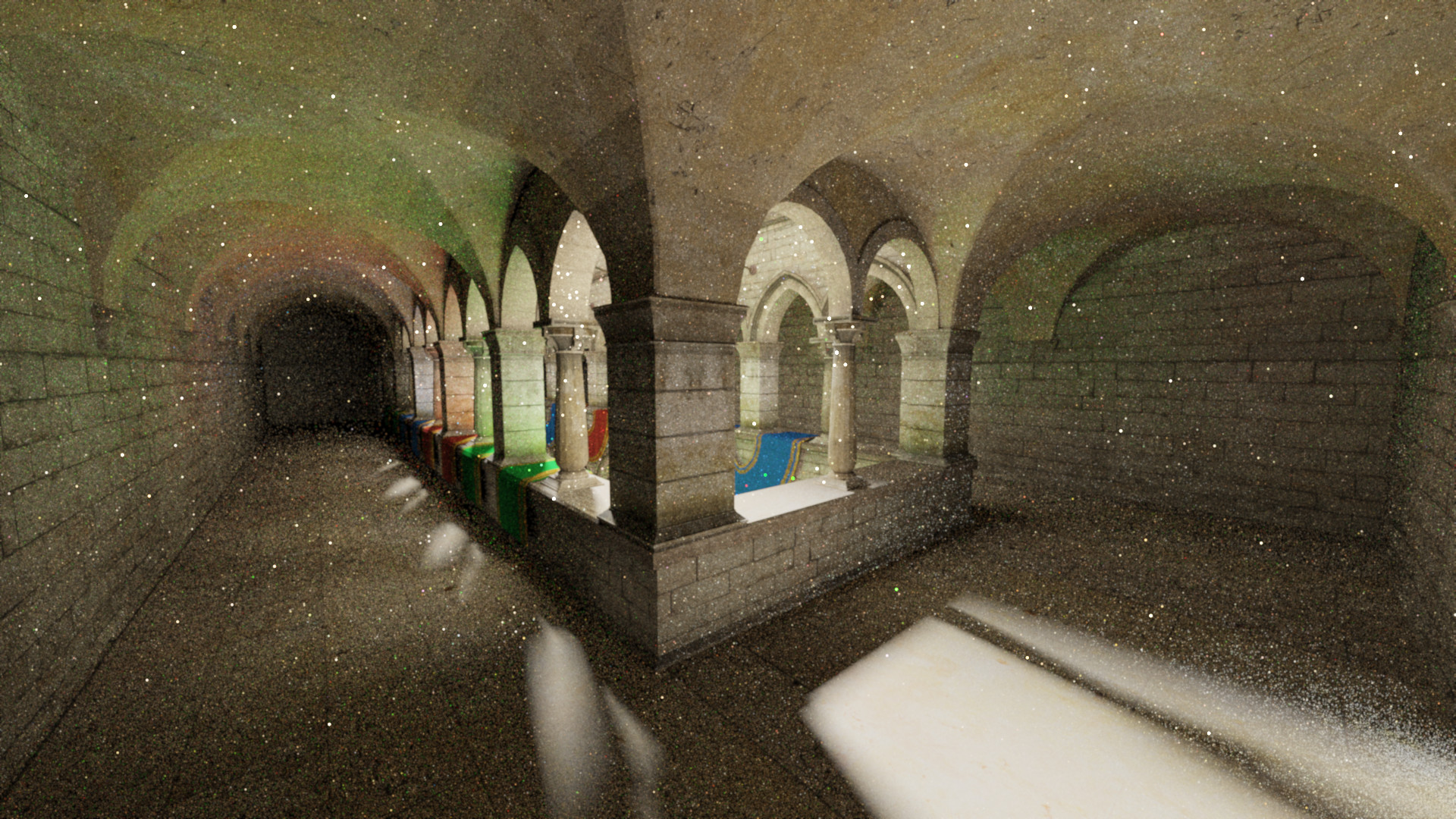
There's a problem here though; with plain BDPT we could have eye- and light- paths with dozens (if not hundreds) of bounces! If we don't choose to place an arbitrary limit on the number of bounces, we end up with an exponential growth of connection rays!
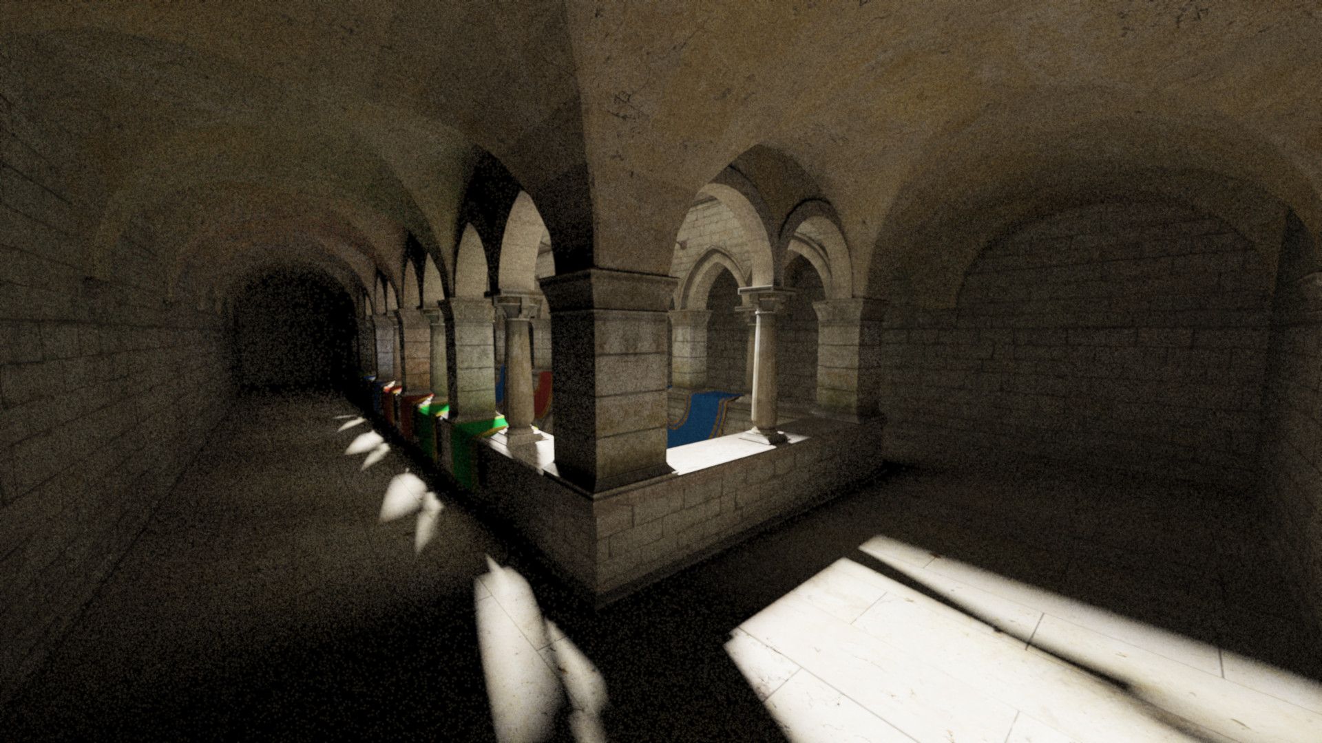
How can we prevent this? The answer is MIS, which if used properly, not only fixes our complexity problem, but also produces a similar result in much less time.

As previously stated, MIS is a way of combining sampling techniques, but by what means?
Multiple-Importance Sampling was a concept discovered by Eric Veach and
Leonidas Guibas in their '95 paper:
Optimally Combining Sampling Techniques for Monte Carlo Rendering.
Veach later expanded on this class of algorithm in his '97 thesis paper:
Robust Monte Carlo Methods for Light Transport Simulation.

In his thesis he explained different use cases for this "adaptive" multi-sampler.
The simplest approach to MIS is to take multiple functions (ie: light-sampling methods), and calculate the contribution each would make if they were to succeed. For each function, you would store it's output as a weight, and then accumulate that weight to a running total.
After all the sampler values are computed, you normalize them by dividing each by the sum of their weights.
The actual sampling consists of selecting which rays will actually be cast by comparing each corresponding weight against a random number (between 0 and 1). This results in lower contribution samples being "culled" out, while following through with brighter samples.
Additionally each iteration contributes less to the scene, but also takes considerably less time to compute as well.

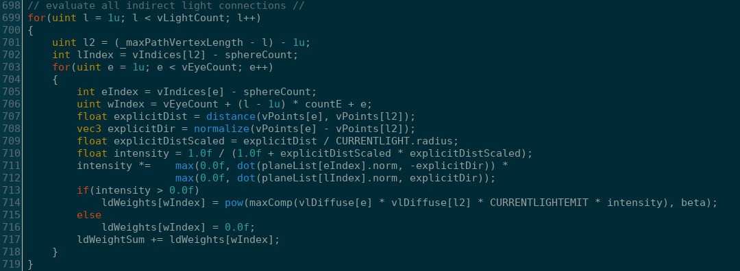
But how do we apply this to BDPT? Well, we just calculate all the ways that every eye-vertex could connect to each light-vertex and sum their weights. Then we take the normalized weights and test them against our random number generator to decide which connection paths are chosen.
If a connection is unoccluded, we add the appropriate contribution of that path divided by the probability of choosing that connection.
Using this method, we reduce our complexity greatly as the path length increases.

So, how do we adapt this algorithm into an actual program? Well, we might start by dividing the process into two parts:
one function for Eye-Tracing, and another for Light-Tracing.
That way we can run them as two independent steps. Then we would make a third function that generates and tests the connection paths.
In both the naive and multiple-importance versions, we can reuse the first two functions. Then we just have to substitute a different path-connection stage depending on which method we select.
In the previous section, I mentioned having to pre-calculate all of the possible connections, and summing their corresponding weights together. This can be efficiently achieved by pre-allocating fixed-size arrays that are passed to every work-thread. Each thread then has a way to store path and connection data per sample.

With most path-tracers, we tend to split light into three separate categories:

• Diffused Light (scattered/re-emmited)
• Specular Light (reflected, normally wavelength independent)
• and Transmitted Light (refracted, possibly attenuated based on depth)

There's also a variation of this model that takes Sub-Surface Scattering (like skin or wax) and Participating Media (like smoke or clouds) into account.
For simplicity's sake, I'm going to ignore these, but you should be always aware of your lighting model when implementing different sampling strategies.

When we generate our eye or light paths, we probabilistically pick one of these lighting methods each time we hit a surface. Additionally, we store an ever diminishing contribution that each of those three could give.
This lets us collapse a traditionally complicated ray-tracer problem into a simple probability-based path-tracer. We can extend this concept further to accommodate our path-vertex and path-connection calculations along with their respective storage as well.

But how many vertices should we allow a path to contain? Or how many connections can a single sample consist of?
Well, in my case, I calculated that 256 bounces would let even highly relective surfaces converge to the rounding-error of a 24-bit image.
That being said, I would suggest calculating the total storage of your sample data, and testing which path-length makes the most sense from a performance vs. accuracy perspective.

For each path-connection that is found to be unshadowed, we calculate the appropriate contribution for it and then accumulate it in our image sample. Then, when all the samples have been calculated, we run our reconstruction filter over them and add it to our current image-buffer.

It's worth noting that special care must be taken when calculating not just the proportional weights, but also the inverse weighting as well. Failure to properly balance sampler functions can lead to very odd results.

Uni-directional render (Left) and bi-directional render (Right) altered to illustrate error.

In my case, I ended up inadvertently canceling-out the material intensity in the sampler. This resulted in directly-lit surfaces being completely uniform in brightness. I also had a similar weighting issue that caused indirect lighting to out-weigh direct lighting!

Same as before, but with the bi-directional render (Right) unaltered.

For the record, these images were rendered with the same settings, but with different rendering methods.
The exposure of the top-right image was darkened to match its UPT counterpart, while the bottom-left is the same render but with the original exposure.

Now, what if we want to run our path-tracer even faster? We can port it to the GPU!
This has a lot of exceptional benefits: massive parallel computation, extensive hardware-accelerated math and image operations, and near instant code compiling.
Actually, writing code to run on the GPU isn't really the hard part.
However, writing efficient code on the GPU is a completely different matter.
If we want to do that, we'll need to re-think how we approach the problem, and most assuredly make compromises.

The first limitation is that we don't have the same level of RAM as the CPU.
GPUs may have similar global memory to a CPU in total capacity, but significantly less cache to utilize per core.
The memory model on current GPUs is based on having many compute-cores (also referred to as "thread-schedulers"), with each of these cores containing many parallel compute lanes.
The processor die contains a unified global cache accessible across the whole device,
with an additional shared cache allocated to each compute-core.
Finally, the lanes themselves have their own local cache which is only accessible by that particular unit.
This three-level memory model can get quite confusing to optimize for. However, we can make it easier by limiting the computation at each step, and reducing the memory that each thread uses.

To start, we can limit paths to have a much smaller vertex count (ie: 8, 16, 32, etc...);
that will result in a much smaller memory limit for path and connection data.
We may also want to change how our data is stored for light-transport.
If we have variables used with each other in a ray, path or connection, then we might want to group those into separate structures.
This optimizes memory access for better cache-efficiency.

GPU-specific storage types can be exploited too.
If a certain process needs many variations of a data-structure, or if it needs to interpolate between them, then you can try storing it in a texture with a sampler.
Using texture memory on the GPU used to be faster, but I am unsure of its advantage on modern GPUs.

Depending on your compute language of choice (OpenCL, CUDA, or GLSL/HLSL), you probably have some kind of control over how your variables are stored in a kernel.
By default, a variable will be local to that thread. However, you can also mark a variable as shared or even global in some scenarios.
This can benefit code that reuses the same data across many threads (assuming that those threads are running nearby).

Of additional importance (at least to code complexity) is Wavefront Path-Tracing.
Using this method you break up your rendering procedure into many smaller kernels, or "wavefronts".
This creates a custom pipeline that supposedly reduces register pressure, and improves performance through reduced execution divergence.

Up to this point, I haven't personally found a way to exploit this for improved performance, but extending the functionality of the renderer is much easier. Due to the modular nature of this model, you can also swap out parts of the pipeline in-place, or remove them entirely.
Refer to: Megakernels Considered Harmful and OpenCL Path-Tracing Best Practices.

With all that out of the way, I hope this article gave some insight into how advanced path-tracing works, and also how its theory is adapted to code.

In my GLSL renderer, I achieved an improvement of around 8-30x that of my previous CPU-based render. I know that even more performance can be squeezed out of my GPU.
Several papers have recorded path-tracing performance exceeding 100 million rays/second on GPUs slower than the one I'm testing on.
Fast Parallel Construction of High-Quality Bounding Volume Hierarchies (2013)
GPU Ray Tracing using Irregular Grids (2017)
Efficient Incoherent Ray Traversal on GPUs Through Compressed Wide BVHs (2017)

In addition, some CPU implementations have greatly exceeded my GPU code in path-tracing performance!
Efficient Ray Tracing Kernels for Modern CPU Architectures (2015)

My gut instinct is that OpenGL compute shaders are the limiting factor of my renderer.
However, I'm skeptical of that as well. Several demos written in GLSL have been released with much higher path-tracing performance than that of mine.
This means that I'm probably overlooking a blatant mistake in my design, or that I'm not using enough data-locality to fully utilize its compute power.

Before I end this article, I feel it should be mentioned that I developed my path-tracer backwards. I should have started by writing a BDPT on the CPU, and testing the correctness of that code. Unfortunately, I decided to just add the required functionality to my GPU-based renderer first.
This was a mistake, preventing me from easily debugging the code, and having no idea where functions were reading or writing to memory.
Also, it meant that if I didn't verify my code extensively enough, I could actually trigger a full system lock-up from the shader!
That's not fun, and it would have saved a tremendous amount of time if I had just adapted working CPU code to the GPU to begin with.

Copyright (c) 2019 David Williams